Excel 2016 Basics Chapter 7
In this tutorials we will cover Basics of excel 2016 like Deleting rows and columns, Hiding rows and columns, Aligning data and Cells, Adjusting text and Text orientation.
Delete rows and columns
Excel allows you to delete rows and columns which you don’t want to be present inside the worksheet. You can delete them by using one of the two different methods. I will show you how to do it in the following example.
Example 1:
First, delete rows: 3 and 4.

Select cells E3 and E4 (or other that are inside row 3 and 4), then go to HOME >> Cells >> Delete >> Delete Sheet Rows.
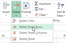
Rows 3 and 4 have been deleted.

To use the second method, select those two rows by clicking and dragging their numbers, then use right-click and select Delete.
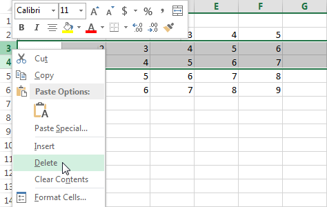
You can delete columns in a similar way.
Hide rows and columns
In some cases, you may want to hide some rows or columns. For example, those that are used only for calculations, and there is no need to see them in your worksheet.
From a technical point of view, hiding columns and rows is actually reducing their size to a minimum. When you hide a row or column, width or height are set to 0.
Hiding
Let’s use the example from the previous lesson.
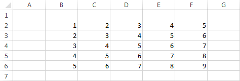
Example 1:
Select rows 3 and 4 and hide them, choosing one of the following methods:
- HOME >> Cells >> Format >> Hide & Unhide >> Hide Rows.
- Right-click the selected rows and choose Hide.

Now, the rows 3 and 4 are hidden.
Unhiding
You can unhide these rows using one of the two methods. First, you have to select rows that are located above and below the hidden rows. In our case, it will be rows: 2 and 5.
Select them and use one of the following methods:
- HOME >> Cells >> Format >> Hide & Unhide >> Unhide Rows.
- Use right-click, then click the Unhide button.
You can deal with columns in the similar way as you deal with rows.
Align data in cells
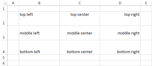
You can align data in cells both horizontally and vertically. Depending on the data you insert inside a cell, Excel aligns it differently. If you enter normal text, then it will be aligned to the left. Any other values, such as numbers or dates will be aligned to the right.
If you increase the height of the row, you will notice that by default, data is also aligned to the bottom.
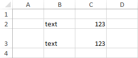
In order to change the alignment of the data inside cells in a way you find useful, choose one of the alignments buttons in HOME >> Alignment.

The three top icons are used to align data vertically, and the three below them are used to align it horizontally. It gives us nine combinations.
Text indent
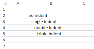
Besides text alignment, Excel also allows you to decrease and increase the text indent. Text indent is used to increase the margin between the text and the left edge of the cell. The icons that are responsible for that are located to the right of the horizontal text alignment icons.

Example:
Look at the following example. The increase indent button was clicked once in cell B3, twice in B4 and three times in B5.
Fit text in a cell
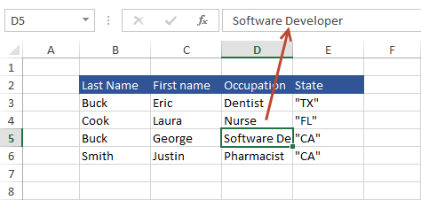
If the text you entered in the cell is too long to display it in its entirety, Excel will display only a part of it. When you click the cell, you can see much more in the formula bar.
There are a few different ways in Excel to display the entire text. Depending on the situation or certain restrictions (for example those imposed by the company you work in), you can choose one of the three methods to achieve this goal.
Changing the width of a column
Example 1:
Widening a column is the easiest and probably the first method that comes to mind. Move the border between cell D and E, so that the cursor will change its shape, as shown in the following picture.

Click the border between cells D and E and drag it to the right, so it is wide enough to contain the entire contents of the cell.
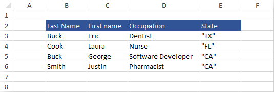
You can also use double-click on the border. When you do it, the column will be widened exactly to contain the widest text in the column.
Text wrapping
When the text is too long, widening columns doesn’t seem to be the best idea because the column would be too wide to scroll the worksheet comfortably. Besides, it would take many pages to print such a document.
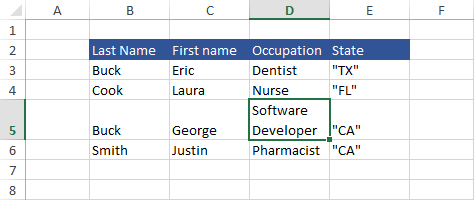
The next method is called Text Wrapping. It will wrap the text and display it in multiple lines, increasing the row height.
Example 2:
Select column D5, then go to HOME >> Alignment >> Wrap Text. In our example, the row becomes twice as high to display the entire text.
Text shrinking
There is another method that allows you to fit the whole text into the cell. In this one you don’t need to change the row height or column width, just adjust the font size.
To use this method, select the cell, then go to HOME >> Alignment and click the little square in the lower right corner. In the new window, select Shrink to fit and press the OK button.
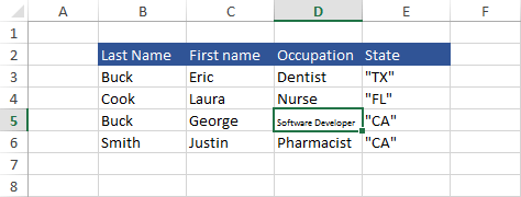
The disadvantage of this method is that it makes sense only when the text is only slightly larger than the column width. Otherwise, the font will be too small and, therefore, impossible to read.
Text orientation
Besides horizontal text orientation, you can also display text vertically or at an angle.
You can change the orientation of the text go to HOME >> Alignment >> Orientation.
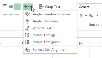
In the drop-down menu, you will find 5 default text orientation types. Three of them are vertical and two diagonal.
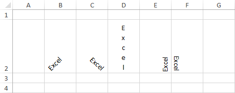
If you need more control over the text orientation, click the last item in the list- Format Cell Alignment.
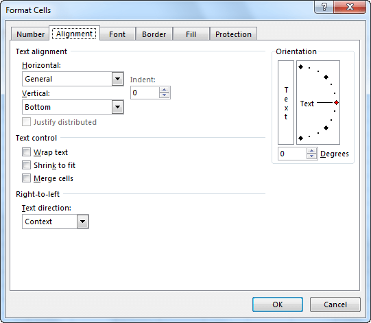
On the right side of the box, in the orientation area, you can set text orientation with an accuracy of one percent. Look at the following examples.

In next tutorial i will Write about Basics of excel 2016 like Color, type and font size, Bold, italic, underline, and strikethrough, Filling cells, and Cell borders. Hope that it helps for you guys.


